1GOVERNING EQUATION
Since the integral and differential forms can be derived from each other, we shall use integral form directly in order to establish our finite volume scheme.
?(1) Continuity equation
Consider the general case in which control volume is neither a fixed volume nor a material volume. The surfaces of the volume are moving at , but not with the local fluid velocity
 . I n such a case, the mass conservation law can be formulated as:
 ?(1)
?(1)
On the right hand side, the first term represents the rate of change of mass included in the control volume. The second term represents the mass flux flowing through the surface of the control volume. Where, is density of fluid,
 is velocity,
 ?represents control volume surrounded by surface S.
(2) Momentum equation
 (2)
(2)
Where ?represent body force per unit volume, stress tensor respectively. In essence, momentum equation is an integral statement of Newton's law for moving control volume.
If Boussinesq’s eddy viscosity concept is adopted, the stresses are determined by
(3) Suspend sediment transport
Conservation law for sediment transport is written as:
 (3)
(3)
Where, C is the local salinity of sediment, and d is the turbulent diffusion of salinity, when only isotropic is considered.  ?is settling or fall velocity because of? the difference between ?specific weight of water and sediment particles. From a viewpoint of multi-phase, this is an assumption of linear superposition about sediment transport
In the equilibrium state, the power of flow to entrain suspended soil particles is quite important parameter. Various non-dimensional? ?formulas had been proposed for this parameter, we adopt the Zhang’s formula (1961) to compute exchange of suspended sediment near bed as boundary condition for Suspend sediment transport.
 (4)
(4)
Where is called entrain power, u is depth-averaged velocity,
  represents gravitation, hydraulic radius, and settling velocity, respectively; K is a coefficient, and m is an exponent. Although Zhang’s formula is defined by depth-averaged suspended-load concentration at each vertical line, this formula has been widely used for 2D case and well calibrated in China.
2.DISCRETIZATION AND ALGORITHM
The momentum and transport conservation law can be expressed in the following unified form:
 ?(5)
?(5)
Here,

represents velocity vector and other transport variables such as sediment, tempter and other contaminants, and  is effective convective velocity. ?And, (5) is solved with finite volume method.
Due to the flexibility of the unstructured mesh, the complex boundary can be accommodated and the size of meshes can be changed according to the topography. Another potential application of the unstructured mesh to the marine system modeling is that it can increase the resolution in the interested area. This can be used to catch the front where the large gradient of the physical parameter appears, such as tsunami.
…

Fig.1 Descretization with multi-layer in vertical direction and definition of transport variables.
Fig.2. unstructured surface grid in horizontal view
The finite volume is shown in Fig.1 and Fig.2. Multi-layers are used in vertical direction, with the bottom surface fitted with bed topography and top surface face fitted with free surface. Transport variables are defined as integral average of finite volume in the middle of layer. Unstructured surface grids are adopted in horizontal view, while the boundaries of finite volume are composed by links between center of element and middle of element boundary. This type of descretization can be named as finite-element-based finite volume method. In fact, the data storage structure is adapted from a early 3D finite-element N-S solver (Jin, 1997).
For the computation of flux across finite volume boundary, convective upwind scheme is used, and MUSCL-Type high-order method is used to construct high-resolution scheme in unstructured grids. On the bottom surface, stress is computed by Cezzy formula for momentum equation, and non-equilibrium formula is used to compute exchange between bed sand and flow for sediment transport equation. On the free surface, stress boundary condition including atmosphere pressure condition and shear stress by wind can be directly introduced.? A semi-implicit scheme is used with pressure correction method for velocity-pressure decoupling. It should be noted that when only one layer is used, the present scheme changes to conservative depth-averaged shallow water model naturedly.
3. VALIDATION WITH ANALYTIC SOLUTION
A few analytic solutions are available for validation of free surface flow. Here, The Long wave resonance in a parabolic basin is given here to validate the ability of the model to capturing wet-dry boundary.
The long wave resonance to be considered takes place in a basin described by a paraboloid of revolution given by
Where,  ?is the still water depth in the center of the basin,
  ?is the distance from the center point,
  ?is the still water radius.
In such a basin, assuming a parabolic free surface, Thacker (1981) based on nonlinear shallow water equations, derived the following analytical solutions for the free surface elevation:

Where

 is the initial wet radius and

is the angular frequency.
The model is tested using the physical values with  =1m,
=1m,  =2500m, and
  =2000m. in the numerical experiment, horizontal grid spacing of
  80m and a time step of
  =
= /240 are employed. Only one layer is adopted here. The non-hydrostatic terms are not included in this calculation.
Figs. 3 and 4 show the time series of the computed and the analytical values of the free surface elevation and velocity, respectively. The comparison of free surface elevation between the numerical and analytical solutions along the  =0 cross section is shown in Fig.5, which begins at the second oscillation and covers a half-period. Good agreements are obtained by the present model, demonstrating the accuracy of the wet-dry boundary algorithm.
Fig.3 Comparison of time series of free surface water level at location (x, y) = (1000, 0).
Fig.4 Comparison of time series of velocity at location (x, y) = (1000, 0)
Fig.5 Comparison between computed(solid line)and analytical(dots)free surface profiles along y=0 at t = (a) 2T, (b) 13/6T, (c) 7/3T and (d) 5/2T.
4. VALIDATION WITH EXPERIMENTAL DATA
Three examples are presented here to show the ability of the present 3D model dealing with discontinuous free surface, short wave transformation and sediment transport.
(1) Non-symmetric dam break in a pool with a pyramidal obstacle
The physical model was built at the Hydraulic Lab. of CITEEC (Spain) under the super vision of J. Puertas. The model consists of a closed pool separated in two parts by a solid wall where a gate (dam) is located in a non-symmetric place.
Fig.6 shows the comparison between experimental data and numerical results on the time evolution to water level during 20s at the measuring points in the pool. The numerical results agree well with the experimental data.
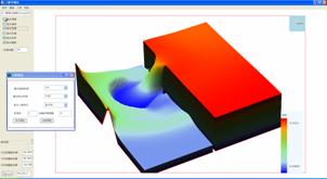
Fig.6 a 3D non-symmetric dam breaking in a pool with a pyramidal obstacle.
Fig.6b experimental data and numerical results on the time evolution to water level during 20s at the measuring points.
(2) Wave transformation over an elliptic shoal Fonts and captions
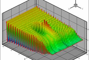
Fig.7a Wave transformation over an elliptic shoal
Wave propagating over three-dimensional complicated bathymetries is a long-lasting problem in coastal engineering. Wave transformation over a submerged elliptic shoal is one of the classic examples to evaluate numerical models for simulating shoaling, refraction, diffraction, and wave focusing processes. Experimental data by Berkhoff (1976) and Vincent and Briggs(1989) have been widely used to validate the Laplace’s equation models and numerous depth-integrated models. These developed 3D non-hydrostatic models can effectively resolve free-surface wave motions using just two vertical layers to reduce the computational cost to an acceptable level.
Fig.7b Comparison with experiment
(3) Modeling of sediment transport in a channel bend with unsteady flow
The laboratory data used to validate the present numerical model were collected by Yen et al. (1995). The experiments were conducted in a laboratory channel bend having a central angle of 180. a radius of curvature along center bend line of rc = 4m, and a width of B = 1m. The base flow was set at Q0 = 0.02m3/s, corresponding to a base flow depth of h0 = 5.44 cm, a mean velocity of u = 0.38m/s. The sediments were specified by the initial median diameter of d50 = 1.0mm and their standard deviation of σ0 = 2.5. The initial bed slope was S0 = 0.002. Bed topography and transverse sediment sorting were investigated.
Five experiments were performed, each having the same initial sediment-size gradation but different inflow hydrographs. At various bend sections, bed elevations were measured and bed surface sediments were sampled at the peak and the end of the hydrograph in each test. Figures 8a, 8b, and 8c show contour plots of the bed deformations and median sediment sizes in plan view compared to the measurements. The contours are displayed in dimensionless form. The bed deformations were normalized by the initial water depth of h0 = 5.44 cm, and the median sediment sizes by the initial median sediment diameter of d0 = 1mm.
The results indicate that bars always evolved at the inner bank while scour was generated at the outer bank. As a consequence, lateral sorting processes occurred with the largest intensity around 90?, indicated by diameters larger than d50 at the outer and smaller than d50 at the inner bank. The maximum deposition height was found between 75? and 90?, and the maximum scour depth occurred between 165? and 180?.
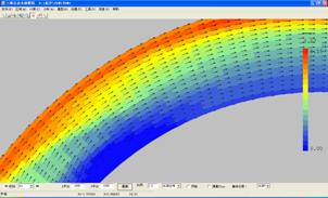
Fig.8a Distribution of velocity
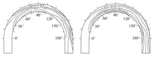
Fig.8b Plan view of measured bed deformations data ; (a)CASE1 ?(b)CASE4
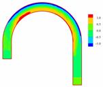
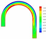
Fig.8c Plan view of ?the present simulation of bed deformations data  ; (a)CASE1 ?(b)CASE4
5. VALIDATION WITH FIELD MEASURED DATA
The Bohai Sea is a semi-enclosed sea, connected with the Huanghai Sea. The tidal wave from the Huanghai Sea propagates through the Bohai Strait into the Bohai Sea. In Bohai Sea, the tidal movement is one of the prominent hydrodynamic processes. In the model, the tide process from 14:00 October 27, 2004 to 15:00 October 28, 2004 is imposed at the open boundary. There are 6973 nodes complete with 13221 triangular meshes. Two layers are chosen vertically with the layer thickness of 25 m, 42 m, respectively from the surface to the bottom. The time step is 10 s. Figs.9b-9d shows the water surface elevation comparisons at three gauging points. It can be seen that the numerical model is reasonable and can be applied to study the tidal currents in Bohai Sea.
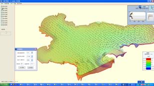
Fig.9a The Bohai Sea overview
Fig.9b Comparison of ?water level at Bayuquan Station.
Fig.9c Comparison of water level at Jinzhou Station.
Fig.9d Comparison of? water level at Jingtanggang station.
6. APPLICATION AND HYDROINFO SYSTEM ESTABLISHMENT CITATION AND REFERENCE LIST
The 3D model has been incorporated into the HYDROINFO System developed by Dalian University of Technology, which has been applied by several institutions of The Ministry of Water Resources and The Ministry of Transport of People’s Republic of China. Fig.10 shows an example of multi-dimension coupling application in Pearl estuary.
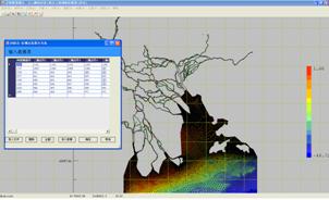
Fig.10a Multi-dimension coupling for Pearl estuary
Fig.10b Discharge comparison in Maco Station
